How to Break the Scaling Wall

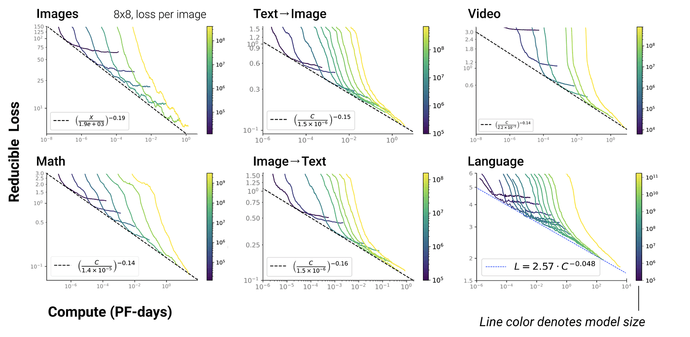
When researchers plot model cross-entropy loss against compute on a log-log scale, the result is a near-straight line: loss falls predictably as compute, model size, or training tokens increase. That empirical regularity - the scaling law - lets teams forecast returns, but it also shows the limit: buying more GPUs gives diminishing marginal returns.

DeepMind's compute-optimal work later showed that, for a fixed compute budget, training more tokens at the right model size can outperform simply increasing parameter count. That is why tokens and data hygiene matter as much as raw model scale.

Those two facts set the problem we care about. The engineering question is not whether the scaling law exists. The question is how to shift the intercept of that log-log line so the same FLOPs buy lower loss. Below I outline the mechanisms that reliably move the intercept, give a one-week playbook you can run on any stack, and explain what we're building at RightNow AI.

What actually moves the intercept

1) Make every token more informative - data hygiene and targeting. Remove duplicates and low-value text. Score and weight high-signal examples. Generate small, targeted synthetic datasets aimed at real failure modes rather than dumping random synthetic text into training. These steps increase sample efficiency and raise the effective value of each training step.

2) Raise effective capacity without linear FLOPs - algorithmic tricks. Conditional compute (sparsity, MoE) activates only the parameters you need per token. Low-rank adapters (LoRA) let you fine-tune capability with far fewer trainable parameters. Practical quantization (e.g., 4-bit workflows) reduces memory and bandwidth costs while preserving accuracy. These techniques change the constants in the scaling law: the slope stays, the intercept drops.

3) Squeeze the hardware - systems engineering that converts paid cycles into useful progress. Profile real runs and fix the hot paths. Replace IO-heavy attention with IO-aware kernels (FlashAttention), fuse kernels to eliminate extra copies, optimize memory layouts, and tune your mix of pipeline/tensor/data parallelism. Memory sharding (ZeRO) reduces per-GPU memory pressure and communication stalls. These fixes turn idle or blocked cycles into FLOPs that actually reduce loss.

Stack those three groups and you lower loss for the same FLOP budget - effectively shifting the whole line downward on the log-log plot.

Scaling visualization

Loss (log)
  |
  |\
  | \\
  |  \\\    original scaling (Kaplan-style power law)
  |   \\\
  |    \\\     ← after systems optim (FlashAttention, ZeRO)
  |     \\\
  |      \\\   ← after algorithmic optim (MoE, LoRA, quant)
  |       \\\  ← after data optim (dedupe, targeted synth)
  +------------------------------------ Compute (log)
     C0     C1     C2     C3

Interpretation: The slope (the scaling exponent) remains. Data, algorithm, and system interventions lower the intercept - same compute, lower loss.

Where paid compute is commonly lost (measure first)

Typical waste breakdown (illustrative)
+-----------------------------------+
| Duplicates / low-value tokens : 30% |
| Kernel inefficiencies         : 25% |
| Communication / imbalance    : 20% |
| Checkpoint / IO overhead     : 15% |
| Suboptimal hyperconfig       : 10% |
+-----------------------------------+

Recovering even a portion of these losses can produce the effective output of a much larger cluster.

A one-week playbook (practical - run this now)

• Day 1 - Profile a full run. Capture kernel and communication traces; find the top 3 hotspots by wall-clock time.

• Day 2 - Data hygiene. Run dedupe and quality scoring on a representative slice. Retrain one epoch and compare validation loss.

• Day 3 - Cheap fine-tune. Replace a full retrain with LoRA/QLoRA on targeted failure modes and measure gain per GPU-hour.

• Day 4 - Kernel fixes. Swap a critical operator to an IO-aware implementation (e.g., FlashAttention), fuse kernels, or change tensor layout. Measure wall-clock change.

• Day 5 - Distributed tuning. Apply sharding/ZeRO where appropriate; reprofile and remove imbalance.

• Day 6 - Small conditional compute probe. Prototype a tiny MoE or conditional block on a subset to validate capacity gains.

• Day 7 - Synthesize and iterate. Generate targeted synthetic examples for remaining errors, adapt, and measure.

Always convert improvements into dollars or experiment counts: seconds saved → GPU-hours saved → experiments gained per month.

Quick scientific justifications

• Scaling laws: the empirical power-law relationship across compute, tokens, and model size provides the slope for planning. (Kaplan et al., 2020)

• Compute-optimal tradeoff: Chinchilla shows tokens matter; training at the compute-optimal point often favors more tokens at the right model size. (Hoffmann et al., 2022)

• Systems wins: IO-aware attention and fused kernels reduce wall-clock time dramatically in attention-heavy runs (FlashAttention).

• Algorithmic efficiency: LoRA and low-rank adapters enable cheap fine-tuning; MoE/conditional compute yields large effective models with lower active FLOPs.

• Memory sharding: ZeRO and related sharding techniques let you scale models across nodes without linear memory blowup.